
Even if your A/B tests are well planned and strategized, when run, they can often lead to non-significant results and erroneous interpretations.
You’re especially prone to errors if incorrect statistical approaches are used.
In this post we’ll illustrate the 10 most important statistical traps to be aware of, and more importantly, how to avoid them.
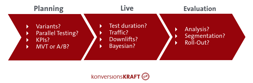
Here’s a quick navigation of what we’ll cover in the post.
Table of contents
I. Statistics traps before testing
Statistics trap #1: Too many variants
Let’s test as many variants as possible; one of them will surely work.
In most cases, testing too many variants at once is not a good idea.
In general, the optimization process should always be hypothesis-driven. Throwing random ideas at the wall won’t get you any where.
There’s another problem with running too many tests: validity— the more test variants you run, the higher the probability of declaring one of them a winner when it really isn’t.
You may already have heard of the “cumulative alpha error” concept.
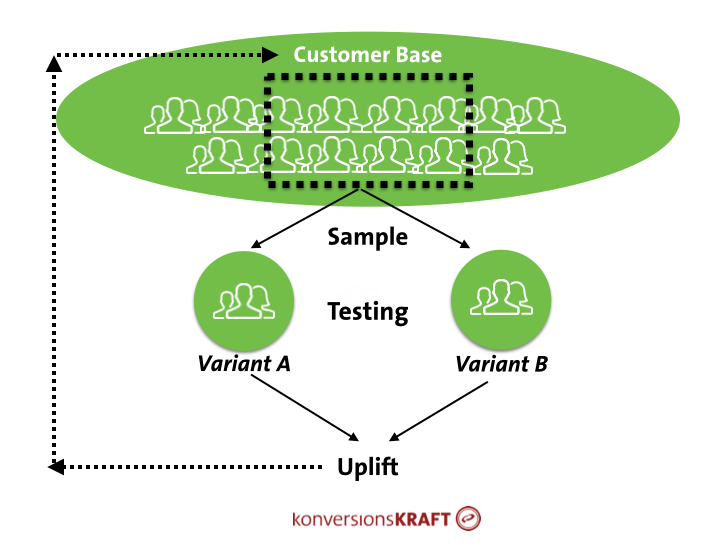
Each test is accompanied by an acceptance of a certain probability of error in the test results. Because A/B testing considers only a part of the entire customer base (your sample), there are always uncertainties of the actual effects.
The goal of the test, however, is to carry-over the effect measured by the test onto the entire customer base which makes confidence in your tests important.
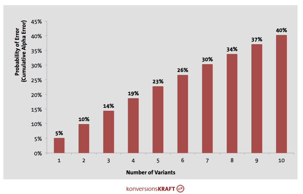
As a rule, we tend to accept a confidence level of 95%. This means that you accept a 5% probability of a type 1 error (“alpha error,” or a false positive). In 5% of all cases an assumption of a significant effect is made, even though in reality there is none at all. This low error probability, however, is valid only in the case of one test variant. It increases exponentially when you introduce multiple variants.
So if you have one variant, the probability of error is 5%, but the cumulative alpha error rises when a number of groups is compared to one other group.
In this case, every individual group comparison has a simple alpha error, whereby this is to be considered cumulatively across all groups (this follows from the axiom of probability theory). For three test variants, each of them compared to the control, the probability of error is already 14%—for eight test variants it is about 34%. This means, for such a test, in more than every third case you find a significant uplift which is the result of chance alone.
You can see how things “escalate” quickly when running a handful of variants at once.
Here’s how you cancalculate the cumulative alpha error for your test:
Cumulative alpha = 1-(1-Alpha)^n
Alpha = selected significance level, as a rule 0.05
n = number of test variants in your test (without the control)
The good news is: If you use the new Smart Stats by VWO or Optimizely’s Stats Engine, the procedures to correct for an increasing probability of error for multiple test variants are applied automatically.
If you have a testing tool that does not use a correction procedure, there are two possibilities:
1. Correct the alpha error yourself
With the help of the statistical analysis of variance (ANOVA), the first thing tested is whether a significant difference exists in the overall comparison of multiple test variants (the so-called F-test). But you still don’t know the test variant for which this is the case. A uni-factorial analysis of variance checks whether the variances of the individual samples differ.
2. Limit the number of test variants
If option one is too complicated or time consuming, the number of test variants can be limited right from the start. Based on our experience, no more than three variants plus the control should be run in one test.
It should be noted that the problem of an increasing probability of error also arises for multivariate testing (MVT)! Practical tips for a successful MVT are found at “Statistics trap #4.”
Statistics trap #2: Estimating interdependencies
No, we can not run two tests simultaneously. The results will influence each other mutually and they distort.
There are different opinions on whether one user should be allowed in a number of tests at the same time.
While some argue that this is not a problem because the effects balance out, others see contamination effects as a result of parallel testing—interactions between tests and variants can lead to non-linear effects, greater variances and sinking validity.
Sometimes there are high levels of interaction effects, and sometimes there aren’t. Here are some different scenarios and what to do:
1. Low risk of interdependencies
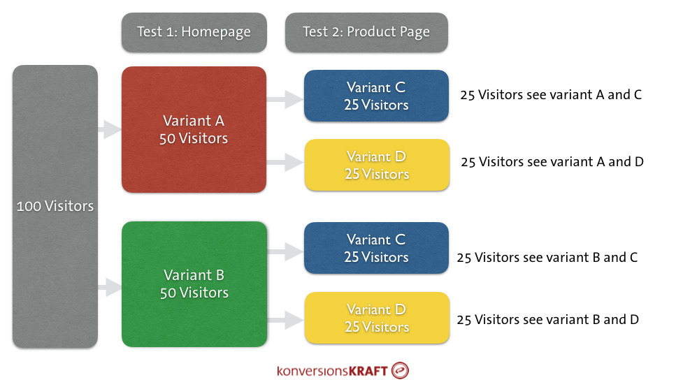
If the risk is low and traffic overlap between the tests is manageable, two tests can absolutely be allowed to run in parallel, so that one and the same user can be in multiple tests.
For example, a concept that tests UVPs on the home page could run in parallel with a test that displays customer opinions on the product page. Both tests can be allowed to run purely methodologically and technically at 100% traffic; that is, one user can be in both tests. The probability that the tests will compete with one another tends to be low here.
Why does this work? Without going into the math of A/B testing too deeply, the issue involves the wonderful randomization principle, which is the foundation of A/B testing.
Users are allocated to the test or control variant by chance. This is true for all tests, including those that run in parallel, allocating the user to multiple tests simultaneously. As a result of this random principle, in combination with the law of large numbers, there is certainty that the share of users who are also participating in other tests is proportional in the test and the control variant. The effects then balance across the measured conversion rate in the groups and uplifts can be measured reliably.
2. High risk of interdependencies
Of course, there are also tests you shouldn’t run simultaneously. In these cases, you usually lack the ability of obtaining valid data for tests on the same page or, especially, on the same elements of a page.
An (extreme) example: In test one you would like to test the placement of the product recommendations on the product page. In test two you change the recommendation engine algorithm, so that you primarily show sales focused articles.
If a user is in the test variant in both tests, the combination of changes can lead to entirely different effects as compared to the user seeing only one of the changes.
There are two solutions for tests that interact strongly:
Solution A: Play it safe; run tests separate of one another
On the one hand, most popular testing tools allow dividing-up traffic to a number of tests. It is possible, for example, to test the placement of the recommendations at 50% traffic, while the other 50% is used for the sale articles in the recommendations. This procedure ensures that the user sees only one of the running test concepts. In this case, you should make sure, that the test runtime is appropriately extended for every test.
If a 50/50 split is not possible, tests can always be run sequentially. In this case, you should always prioritize the tests and accordingly and synchronize them in your roadmap.
Solution B: Multivariate testing
Another possibility is to combine the test concepts to one multivariate test. This makes sense if the test concepts optimize on the same goal and run on the same page.
This means the variants must be reasonably combinable. If one test, for example, is changing the main-navigation and the other is the UVPs in checkout, then it makes little sense because there are hardly any interactions between the concepts.
Statistics trap #3: Click rates and conversion rate
“If click rates increase, then we’ll also notice an increase in the conversion rate.”
Just because you increase visits to the product page, or because visitors place an item in the shopping cart more often, doesn’t mean you’ve increased the macro-goal.
…If only if were so simple!
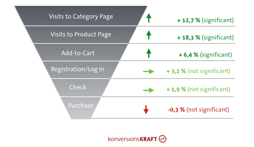
Therefore, it’s crucial to measure macro-conversions in every test.
Selecting and Prioritizing the Main KPI
Of course, your macro-conversion depends on the business, the goal, ad the specific test hypothesis. Here are a few to consider:
Conversion rate
This the most common KPI for an ecommerce shop. If the test concerns primarily converting users to buyers, the conversion rate should have the highest priority.
Shopping Cart Values / Revenue Per Visitor
Revenue per visitor is another common ecommerce KPI, and it’s especially important in a few specific cases.
For example, optimizing product recommendations on the product page (design, placement, algorithm) does not necessarily lead to people buying anything at all. But, presumably, people will buy more when they do finally make a purchase. Recommendations for complementary products (cross-sell), for example, result in an incentive to buy matching jeans together with the new top at the same time. In that case, the revenue per conversion or per visitor is more relevant than conversion rate.
Returns
If, for example, you want to test whether information about size (“tends to run smaller”) on the product page helps the customer finding the proper size, you should go a step further.
Ultimately, persuading customers to buy something that’s going to get returned is short-sighted and a net negative. In this case, measure the revenue after return or the return rate. The corresponding data can be analyzed by connecting the testing tool and the data warehouse (DWH) (see Statistics trap #8).

Micro-conversions as merely diagnostic instruments
Of course, this does not mean that soft KPIs, like click-rates or pageviews, do not matter. However, they should not serve to evaluate the ultimate success of a concept, but rather as diagnostic instruments (article in German).
Assume that you test an optimized variant of the meta-navigation and would like to discover whether customers are buying more. Surprisingly, the results show no changes in conversion rate or the revenue. Are customers using the new navigation exactly like the old one? Or are they using other entry points such as the side-navigation, search, or teaser categories?
In this case it may be helpful to look at the click rates on navigation elements or the use of internal search in the variants. You will come a step closer to the answer to “why” and understand the behavior of your customers.
Tune the test size to the KPI
While running tests you often see that, after a relatively short time, there are already significant uplifts in the micro-conversions, such as the add-to-basket or clicks. But none of this appears in the conversion rate.
In fact, there is a connection between the type of KPI and the required test size. This is due to fluctuations and the uncertainty that vary depending on the KPI: the higher these uncertainties, the longer the test must run in order to verify significant effects.
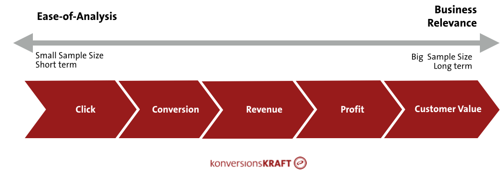
Click-rates or pageviews are so-called count data and have a relatively small range of fluctuation: click or no click.
The conversion rate, however, is quite different. Whether someone actually buys or not is influenced by other factors that lead to an increase in the uncertainties for this KPI.
In order to verify effects in revenue KPIs (e.g. basket size), you need an even bigger sample size than for the conversion rate. Regarding these so-called metric KPIs, there is a high uncertainty about the level of purchasing – if a user buys anything at all.
If you would like to optimize on revenue-after-returns, then the test size should be further increased for better quality data. For this KPI, it is most difficult to make reliable statements.
If someone is buying, then how much are they buying and, if they return things, how much are they returning? The test is more uncertain, which requires a longer test runtime.
To make sure that you are actually getting reliable results, you should first think about the main KPI for your test and then tune the test size appropriately to this. Youd be suprised
Don’t measure too many metrics
The more KPIs you measure, the more difficult the final decision may be.
You should be thinking about which macro and micro-conversions you really need before you start the test. If every metric available in the tool is randomly used to measure, you wind up losing sight of the goal of the test. It’s easier to succumb to cognitive biases, like the Texas Sharpshooter effect, that make it harder for decisions to be made.
Additionally, a very high number of metrics leads to an increase in the probability of finding an effect in a metric that has arisen purely by chance.
Statistics trap #4: Fear of Multivariate Tests
We should not run it as a multivariate test. Much too costly and, anyway, the results are not valid.
The success of a multivariate test (MVT) depends on how you do it. Set up properly, multivariate tests are a great tool to test different factors and combinations. Using one MVT to simultaneously test a number of factors on a page sounds complicated. But it doesn’t have to be. There are only a couple of rules that you should keep in mind…
Do not test too many variants
The problem of cumulative alpha errors also arises if you set up the test as MVT with a number of variants. In order to prevent declaring a variant a winner even when it is not, you should limit the number of combinations here as much as you can.
Based on good hypothesis formation, factors and their combinations should be selected carefully. Additionally, you can work with a higher confidence level (for example 99.5%) in order to make sure that the results are valid.
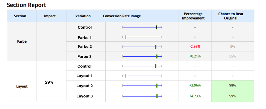
With the results of a MVT, you naturally first check which variant has achieved the highest (and significant) uplift. However, you only get information on which combination of factors achieved this uplift. It’s also important to analyze the influence of individual factors on the conversion rate. This can be done with the help of a so-called analysis of variance. This method isolates the effect of the individual factors (in the example, colors and layout) on the conversion rate.
Validate the results in the follow-up test
To increase faith in your MVT results, you can also validate the test winner by running a subsequent A/B test. You simply run the winning combination against the relevant control.
II. Statistics Traps During Testing
Statistics trap #5: Stopped Too Early
The test has been running for three days already and the variant is performing poorly. We should stop the test.
Many times, there may be good reasons to stop a test early. For example, if your relevant business goals are threatened by a test variant that is performing significantly poorly.
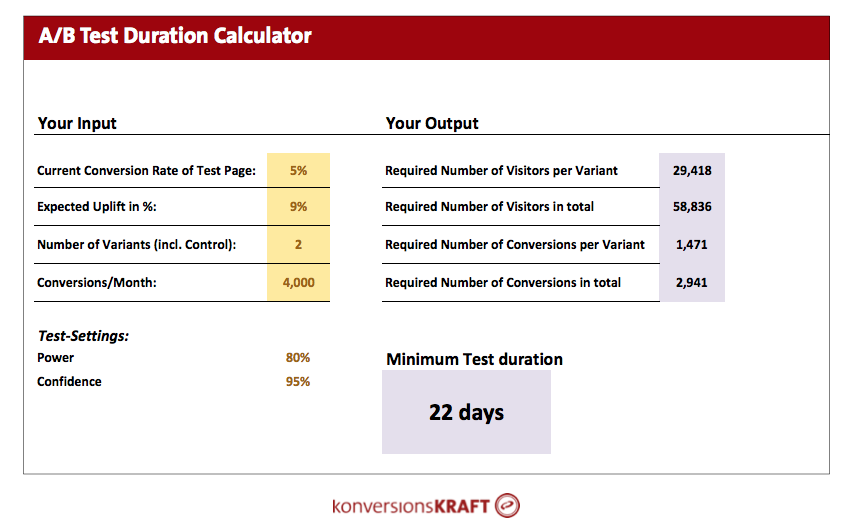
But to decide on the success or failure of a concept requires more than three days of testing. Every test requires a minimum test size (article in german) in order to be able to make any statement at all on whether or not a concept works.
In the first few days of a test, you’ll often notice a wild fluctuation of the results. Since the numbers are small, this could well be the results of chance. Perhaps, purely by chance, a customer in the control purchased so much that the control heads upwards artificially and the test features a temporary downlift (see Statistics Trap #8).
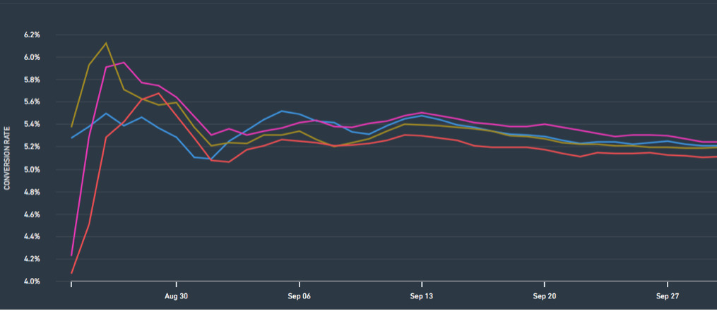
I have often experienced that negative effects at the start can reverse with time, and the test variant shows a significant positive effect after three weeks. Before the test, you should estimate how long a test must run with the help of tools to calculate test duration.
If, at the start, a test shows no significant downlift, this simply means: keep calm for now and continue testing.
Statistics trap #6: Shutting Off Variants
No problem. If one variant doesn’t work, we’ll just change it or shut it off.
If one of your variants is performing so poorly that business goals are threatened, of course you’re going to want to shut off this variant. Similarly, people will often start variants with low traffic allocation and then increase over time (ramp-up). Finally, sometimes people change midway through a test.
All three of the above can distort the results: For A/B testing, the test results are representative of the entire testing time and, that is, in equal parts. If you change the traffic this leads to certain time periods being over- or under-represented.
Shutting off a variant in the middle of the test has the same effect. If the content of a variant is changed, the test result will be a weird mixture of different hypotheses and concepts that finally no longer provides any insight at all.
Here we need to find a healthy balance of scientific rigor and validity & practical business concerns.
Here are some tips to achieve that balance:
- If a variant is shut down as early as the first few days after the start of the test, it is recommended that the test should be started again but without the variant. In this case, the loss of time is not too high.
- Before you change the variants during the test, better to start a new test and test the adapted variant against the control.
- If you change the traffic to a higher level from day to day, make sure that you cover a sufficient amount of time with the maximum desired traffic quantity, whereby the traffic remains stable across the time.
Statistics trap #7: Bayesian Test Procedures
The new Bayesian test procedures get us results much quicker.
The new statistical procedures that have already been applied by VWO and Optimizely provide the advantage that you can interpret the test results at any time and the results are valid even if the required test size has not yet been reached.
However, Bayesian procedures are no protection against incorrect methodology. Or as the New York Times put it, ” “Bayesian statistics, in short, can’t save us from bad science.”
The Problem with Expectations
Before using Bayesian procedures you should make a so-called a priori assumption which factors in the probability at which the test concept will be successful. If the assumption is wrong, there is a risk of long test runtimes and non-valid results.
The Problem With Small Test Size
The results are indeed interpretable at any time during the test, but at the start, when the fluctuations are very high, you should be careful. The number of visitors in the test is still very small and strongly influenced by unusual observations (e.g. very high order values).
Despite the advantages that the Bayesian approach has, the method does not provide adequate validity when the data set is sparse. The newer procedures do not protect from incorrect approaches to A/B testing (by the way, the same is also true of the traditional frequentistic procedures!). No method will save you from bad methodology.
III. Statistics Traps During Evaluation
Statistics trap #8: Trusting Only One Source of Data
Testing tool results are fully adequate to make a decision.
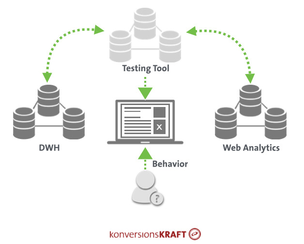
Sure. The testing tool lets us determine whether or not a tested concept leads to a higher conversion rate. But it is often worthwhile to have a detailed look at the data in order to generate more insights and to validate results. Results from the testing tool should not be stored in a data silo, but rather be combined with other databases, such as the web analytics system or the DWH.
Thereby, a series of important questions can be answered:
Why?
The question “why” always arises when the results of a test are not as expected. As in the above-described example on the meta-navigation (see Statistics Trap #3), it can be useful to look at micro-conversions in order to better understand test results.
If you failed to set up clicks on navigation elements or the use of the internal search as goals before the test, such questions cannot be answered later with the testing tool. If, in contrast, your testing tool is connected to the web analytics tool, you can evaluate these metrics.
Will the conversion rate uplift also lead to more profit?
If customers place more orders as a result of an optimization concept, great! If, however, they return the same amount or more, this can eventually mean a financial loss. Connecting your testing tool and the DWH allows your to analyze results after returns. Here, the variant IDs are transferred to the backend, and you can view the return rate or the revenue after returns as additional KPIs in the test and control variant.
Taking bulk orderers into consideration
Almost every online shop has them and usually they cause problems for the valid evaluation of a test: the bulk orderers. This can include call-center customers, customers from B2B, or excessive online shoppers. These so-called outliers can distort results. Why is that? Well, you look at average values when evaluating test results:
- The conversion rate is nothing but the average rate of conversions in a certain group of visitors.
- The revenue per visitor is the average revenue per visitor.
Unusually high values in the number of orders or the shopping cart values push this average value upward. If the control features a customer with extremely high values purely by chance, at a relatively small test size this can already lead to results that are no longer positive, but rather become even significantly negative.
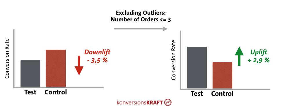
What can you do about outliers? All popular testing tools allow obtaining files with raw data. Here, all customer orders in the variants are listed. Another possibility is to set up corresponding reports your connected web analytics tool of choice, and to exclude abnormally high orders through the appropriate filter setting.

Even through there is some cost, filtering out outliers is worth doing it because you can often discover significant effects that are simply “hidden” by outliers.
For data freaks: the valid calculation of confidence intervals
Traditional methods to calculate confidence intervals include a problem: they assume that the fundamental data follows a certain distribution, namely a normal distribution. The left graphic shows a perfect (theoretical) normal distribution. The number of orders fluctuates around a positive average value. In the example, most customers order five times. More or fewer orders arise less often. The graphic to the right shows the reality.
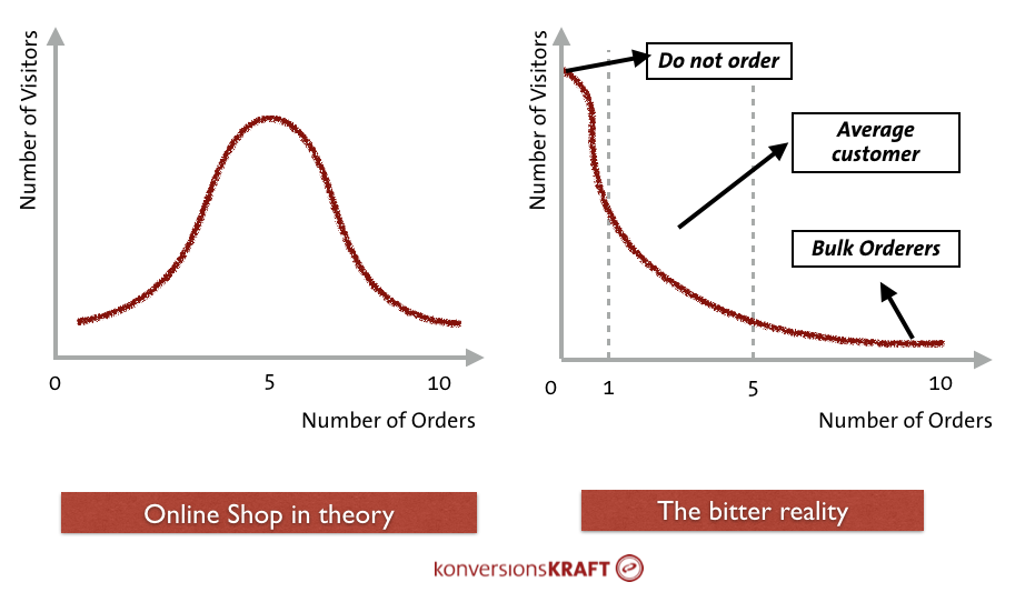
Assuming an average conversion rate of 5%, 95% are customers who don’t buy. Most buyers have probably placed one or two orders, and there are a few customers who order an extreme quantity.
Such distributions are referred to as “right skewed” and they have an influence on the validity of the confidence intervals, especially at a small test size. In essence, the intervals can no longer be reliably calculated. The central limit theorem implies these distortions will carry less weight with very large samples, but how “incorrect” the confidence intervals actually are depends on how much the data deviates from a perfectly normal distribution.
Regarding an average online shop, at least 90% of customers do not buy anything. The proportion of “zeros” in the data is extreme and the deviations in general are enormous (The Shapiro-Wilk test lets you test your data for normal distribution.).
As a consequence, taking a look at the data apart from using the classic t-test is worthwhile. There are other methods that provide reliable results for underlying data that is non-normally distributed.
1. U-Test
The Mann-Whitney U-Test (Wilcoxon rank-sum test) is an alternative to the t-test when the data deviates greatly from the normal distribution.
2. Robust statistics
Methods from robust statistics are used when the data is not normally distributed or distorted by outliers. Here, average values and variances are calculated such that they are not influenced by unusually high or low values.
3. Bootstrapping
This so-called non-parametric procedure works independently of any distribution assumption and provides reliable estimates for confidence levels and intervals. At its core, it belongs to the resampling methods. They provide reliable estimates of the distribution of variables on the basis of the observed data through random sampling procedures.
Statistics trap #9: Evaluation in segments
I am going to look at the results in the segments. I will certainly find an uplift somewhere.
In general, going through your segments is a good idea. A/B test results are, by default, reported across all visitors—but some groups might react differently, and that’s not visible in the aggregate data.
A favorite example is unique value propositions (UVP) – features that make an online shop unique.
It’s common to have varying effects with new and existing customers. While existing customers already know the advantages of a purchase, UVPs help in the process of convincing new customers to buy and to build trust. These varying reactions are not detected in the aggregated reports, and you may be disappointed because no significant uplift can be verified overall.
By connecting the testing tool to other data sources (web analytics, DWH) you can analyze the test results for a series of customer characteristics that are not available in a testing tool, for example:
- Gender;
- Age;
- Categories in which someone makes a purchase;
- Pages visited;
- Data on click behavior;
- Return rate;
- Geolocation.
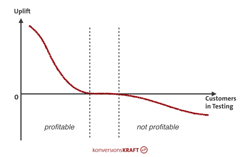
However, caution is recommended here. The probability of error increases exponentially the more segments you compare to one another. Consequently, you should avoid going randomly through all the segments you can think of. They should always remain interpretable, exploitable, relevant to your test concept.
Additionally, you should take care that the segments are adequately large enough.
If, for example, only those visitors are included who access a category page with their tablet, go to a product page, are female and purchase on weekends, this will lead to seeing only a fraction of the visitors.
Therefore, always be careful that the test size is also sufficient in the segments. If you already know before the test that you will do a segmentation of the results, it is recommended that the test duration should be at least doubled. You can verify how certain the results are in the respective segment by using the konversionsKRAFT significance calculator (in german) or CXL AB test calculator.
Statistics trap #10: Extrapolating from test results
The test was probably not so successful after all; we rolled-out the concept, but the conversion rate didn’t go up.
After a successful test, projections are often made regarding the additional revenue that will be generated in the future on the basis of test results. As a result, you see neat-looking management presentations, containing suggestions that a particular test concept will generate a plus in revenue of 40% in the next two years. Sounds great, but is that true?
Sorry for the harsh words, but, please don’t do it! The result of such an extrapolation is as reliable as saying today that there will be rain in three months. You wouldn’t believe that either, would you? To simply predict the result of a test linearly into the future does not work for the following reason:
Reason 1: Short- vs. long-term effects
As a rule, A/B testing measures whether the concept leads to short term changes in customer behavior. The test runs three weeks and you see that the conversion rate increases by x%. So far, so good. However, this change does not say anything about the effect on long-term customer behavior and KPIs such as customer satisfaction and customer loyalty.
To be able to do so, the test would have to run far longer in order to record habituation effects or changes in the customer base and user needs. There’s also the novelty effect to be aware of. Users get used to novelties: what impresses us today is already merely habit tomorrow and is no longer strongly perceived.
Consequently, it is simply wrong to assume the measured short-term effect is a constant and project that holds for the future.
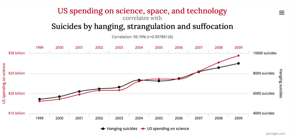
Reason 2: Causality vs. correlation
Assume that the test showed a significant uplift and the test concept is to be solidly implemented. What often happens are so-called before-and-after comparisons, with the goal to find the measured effect in the conversion rate. Here, the conversion rate in the time period before the implementation is compared to a time period after the implementation. It is expected that the difference in the two rates must correspond exactly to the measured effect of the test. Well, usually it doesn’t.
Of course, changes that go live can lead to increases in the conversion rate. However, there are still hundreds of other influencing factors in parallel that also determine the conversion rate (e.g. season, sale events, delivery difficulties, new products, different customers or simply just bugs).
It is important to distinguish between causation and correlation. Correlation only states the extent to which two characteristic numbers follow a common trend. However, correlation says nothing about whether one characteristic number is causal, whether it is the origin of the change in the other variable.
This fallacy is clear the photo below: U.S. spendings for science, space and technology increase and, at the same time, more people commit suicide. Makes no sense, right?
(Image source)
If, after going live, changes in the conversion rate are observed, a single effect cannot be isolated. It is not known which factors are causal for the conversion rate change. Assuming the implemented concept has a positive effect, there can be other negative influencing factors, so that the effect overall is no longer verifiable in the end.
The only possibility of measuring causal relationships and the effect of a test concept in the long term is the following: After a successful test you roll out the concept for 95% of your customers (for example through your testing tool). The remaining 5% is left as control group. By continuously comparing these two groups you can measure the long-term effect of your concept.
If this method is not practicable for you, you will find further tips here to distinguish between correlation and causation.
Reason 3: Misinterpretation of confidence
A further problem is that there are still misunderstandings in the interpretation of confidence.
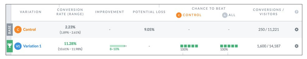
Assume a test shows an uplift of 4.5 % and a confidence level of 98%. That does not mean that the effect is 4.5 % with a probability of 98%! Every confidence analysis provides an interval that contains the expected uplift at a certain probability (confidence). That’s it.
In the example, this could mean that the effect based on the measured values ranges between 2% and 7% at a probability of 98%. It is therefore a fallacy to assume that the actual effect corresponds exactly to that of the test. This interval, however, does become smaller the longer the test runs, but it never arrives at an exact point estimate. The confidence level simply gives an estimate about how stable the result is.
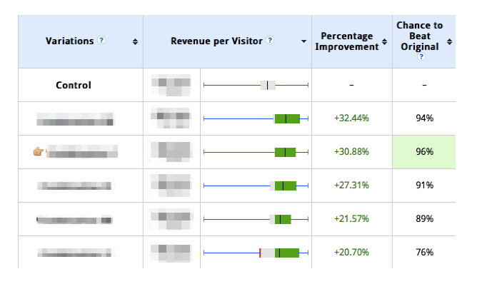
By the way, there is a small but important difference between the confidence level and the chance-to-beat-original (CTBO), which is reported in most testing tools.
The confidence level provides the probability that the uplift is in a certain interval (the confidence interval) and it says nothing about whether a concept is successful or not. The CTBO, on the other hand, measures whether and by how much confidence intervals overlap, and how likely it is that the test variant is better than the control in some way. It is important to know this difference in order to come up with correct test conclusions.
Conclusion
If you rely purely on the numbers from a testing tool, this can lead to errors and may threaten the validity of your results. To avoid this, there are a couple of fundamental rules that should be followed for every phase of the test.
With the topic of A/B testing there is a regular conflict between the scientific demand for validity of a test and actual business needs. You should try to find a good middle path so that your tests always provide practical, relevant results, while you still have enough trust in your test data.
Related Posts
-

A/B testing is highly useful, no question here. But a lot of businesses should not be…
-

As a marketer and optimizer it's only natural to want to speed up your testing…
-

A/B testing is great and very easy to do these days. Tools are getting better…
-
A/B testing is fun. With so many easy-to-use tools, anyone can—and should—do it. However, there's…


Great article! I do, however, have to disagree a bit with some of the parts of #5: Stopped Too Early. While I agree you should set your test sample size in advance and not make any concrete analysis until you’ve hit that sample size, sometimes stopping tests early is the smartest business decision. Always running tests to their predetermined sample size is a luxury that underestimates the opportunity cost of NOT starting a new test with a (potentially) higher chance of delivering a more significant result. Every week you continue to run a test that is unlikely to deliver a significant result for your business is traffic that could potentially be better utilized on other tests.
More often than not we see teams make the opposite mistake–run tests too long because they’re waiting to hit stat sig. This reduces their testing velocity which in turn negatively impacts the performance of their overall testing program. But I suppose thats an operational mistake they are making, not necessarily a statistical mistake :-)