Why create a custom attribution tool? Because with out-of-the-box tools, you’re limited by their functionality, data transformations, models, and heuristics.
With raw data, you can build any attribution model that fits your business and domain area best. While few small companies collect raw data, most large businesses bring it into a data warehouse and visualize it using BI tools such as Google Data Studio, Tableau, Microsoft Power BI, Looker, etc.
Google BigQuery is one of the most popular data warehouses. It’s extremely powerful, fast, and easy to use. In fact, you can use Google BigQuery not only for end-to-end marketing analytics but to train machine-learning models for behavior-based attribution.
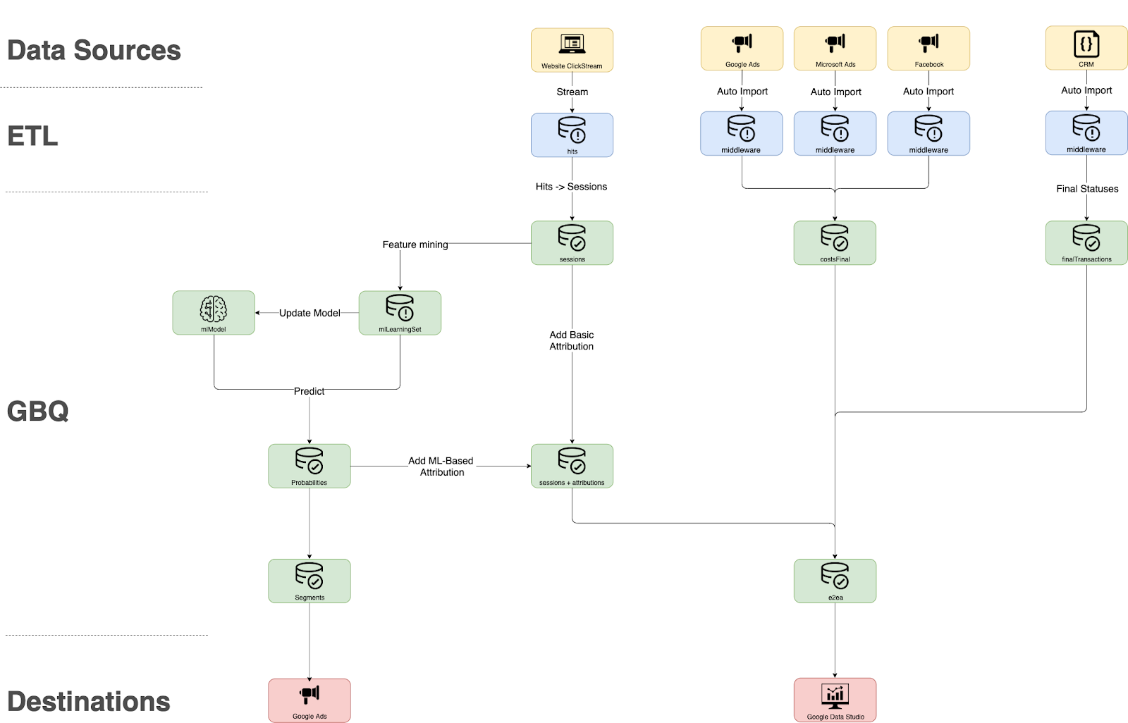
In a nutshell, the process looks like this:
- Collect data from ad platforms (e.g., Facebook Ads, Google Ads, Microsoft Ads, etc.);
- Collect data from your website—pageviews, events, UTM parameters, context (e.g, browser, region, etc.), and conversions;
- Collect data from the CRM about final orders/lead statuses;
- Stitch everything together by session to understand the cost of each session;
- Apply attribution models to understand the value of each session.
Below, I share how to unleash the full potential of raw data and start using Google BigQuery ML tomorrow to build sophisticated attributions with just a bit of SQL—no knowledge of Python, R, or any other programming language needed.
Table of contents
The challenge of attribution
For most companies, it’s unlikely that a user will buy something with their first click. Users typically visit your site a few times from different sources before they make a purchase.
Those sources could be:
- Organic search;
- Social media;
- Referral and affiliate links;
- Banner ads and retargeting ads.
You can see all of the sources in reports like Top Conversion Paths in Google Analytics:
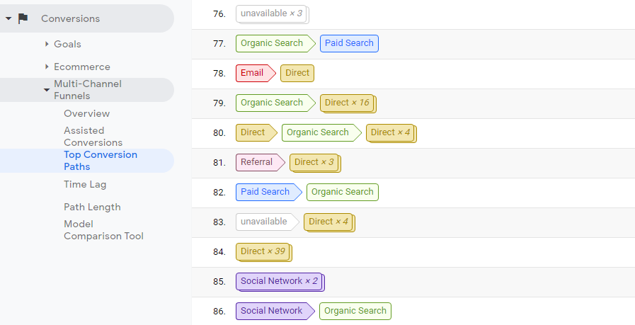
Over time, you accumulate a trove of source types and chains. That makes channel performance difficult to compare. For this reason, we use special rules to assess revenue from each source. Those rules are commonly called attribution rules.
Attribution is the identification of a set of user actions that contribute to a desired outcome, followed by value assignment to each of these events.
There are two types:
- Single channel;
- Multi channel.
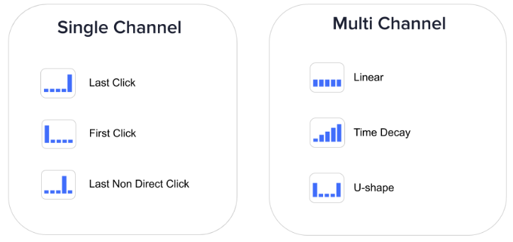
Single-channel types assign 100% of value to one source. A multi-channel attribution model distributes the conversion values across several sources, using a certain proportion. For the latter, the exact proportion of value distribution is determined by the rules of attribution.
Single-channel attribution doesn’t reflect the reality of modern customer journeys and is extremely biased. At the same time, multi-channel attribution has its own challenges:
- Most multi-channel attribution models are full of heuristics—decisions made by (expert) people. For example, with a linear attribution model, the same value is assigned for each channel; in a U-shaped model, most value goes to the first and the last channel, with the rest split among other channels. These attribution models are based on algorithms that people invented to reflect reality, but reality is much more complex.
- Even data-driven attribution isn’t fraud-tolerant because, in most cases, it takes into account only pageviews and UTM parameters; actual behavior isn’t analyzed.
- All attribution models are retrospective. They tell us some statistics from the past while we want to know what to do in the future.
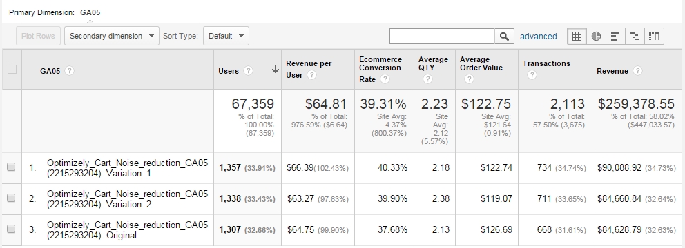
As an example, let’s look at the following figures, which reflect the stats of two November ad campaigns:
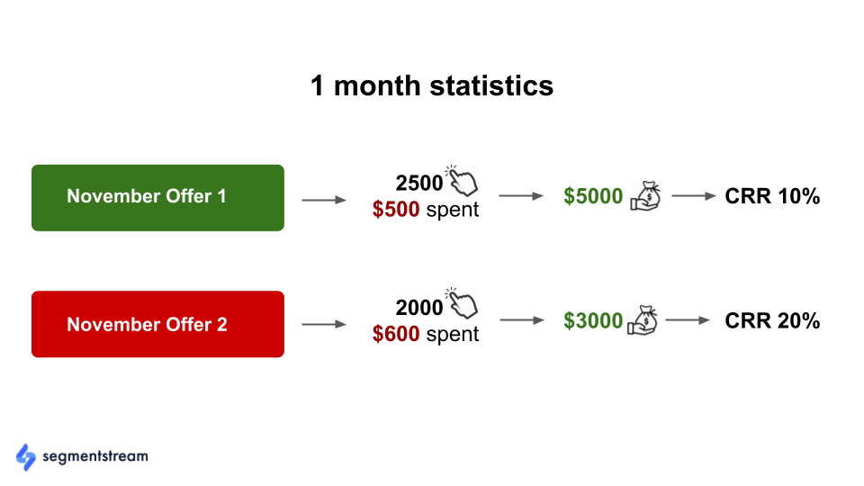
“November Offer 1” performs two times better in terms of Cost-Revenue Ratio (CRR) compared to “November Offer 2.” If we had known this in advance, we could’ve allocated more budget to Offer 1 while reducing budget for Offer 2. However, it’s impossible to change the past.
In December, we’ll have new ads, so we won’t be able to reuse November statistics and the gathered knowledge.
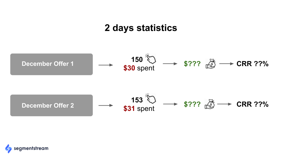
We don’t want to spend another month investing in an inefficient marketing campaign. This is where machine learning and predictive analytics comes in.
What machine learning changes
Machine Learning allows us to transform our approach to attribution and analytics from algorithmic (i.e. Data + Rules = Outcome) to supervised learning (i.e. Data + Desired Outcome = Rules).
Actually, the very definition of attribution (left) fits the machine-learning approach (right):
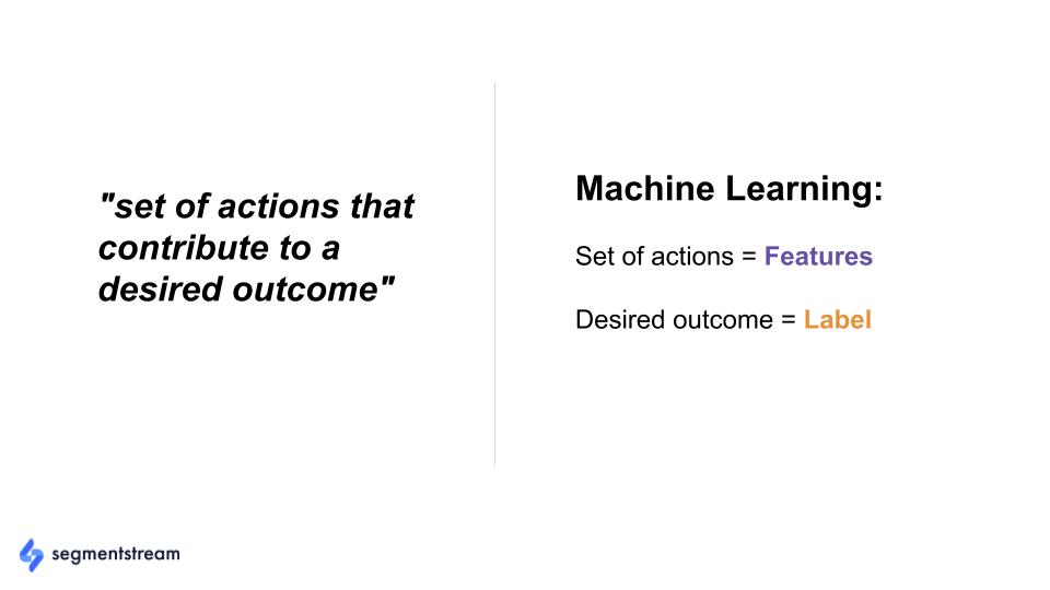
As a result, machine-learning models have several potential advantages:
- Fraud tolerant;
- Able to reuse gained knowledge;
- Able to redistribute value between multiple channels (without manual algorithms and predefined coefficients);
- Take into account not only pageviews and UTM parameters but actual user behavior.
Below, I describe how we built such a model, using Google BigQuery ML to do the heavy lifting.
Four steps to build an attribution model with Google BigQuery ML
Step 1: Feature mining
It’s impossible to train any machine-learning model without proper feature mining. We decided to collect all possible features of the following types:
- Recency features. How long ago an event or micro-conversion happened in a certain timeframe;
- Frequency features. How often an event or micro-conversion happened in a certain timeframe;
- Monetary features. The monetary value of events or micro-conversions that happened in a certain timeframe;
- Contextual features. Information about user device, region, screen resolution, etc.;
- Feature permutations. Permutations of all above features to predict non-linear correlations.
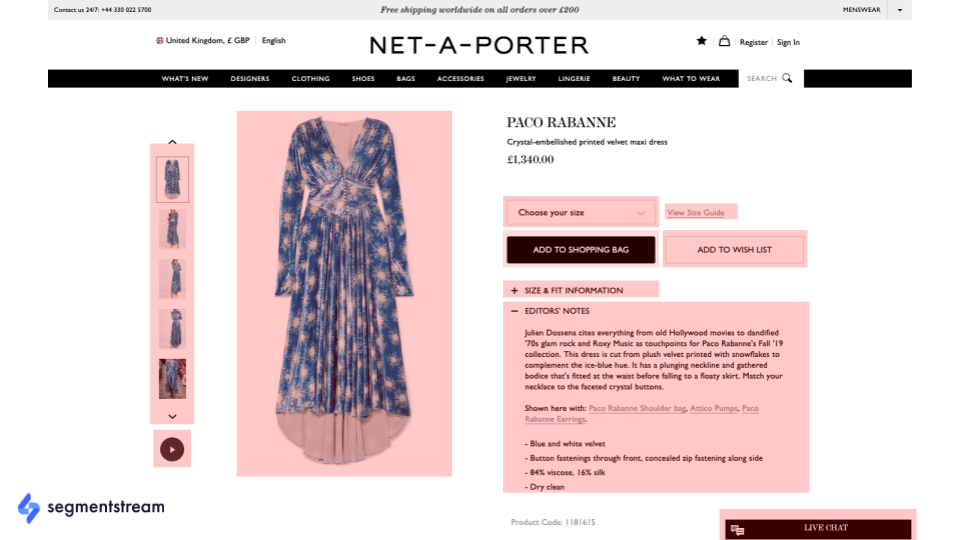
When comparing simple, algorithmic attribution models, it’s important to collect and analyze hundreds and thousands of different events. Below, for example, are different micro-conversions that could be collected on an ecommerce product page for a fashion website:
- Image impressions;
- Image clicks;
- Checking size;
- Selecting size;
- Reading more details;
- Viewed size map;
- Adding to Wishlist;
- Adding to cart, etc.
Some micro-conversions have more predictive power than you might expect. For example, after building our model, we found that viewing all images on a product page has enormous predictive power for future purchases.
In standard ecommerce funnels, analysis of product pageviews with one image viewed is the same as product pageviews with all images viewed. A full analysis of micro-conversions is far different.
We use SegmentStream JavaScript SDK, part of our platform, to collect all possible interactions and micro-conversions and store them directly in Google BigQuery. But you can do the same if you export hit-level data into Google BigQuery via the Google Analytics API or if you have Google Analytics 360, which has a built-in export to BigQuery.
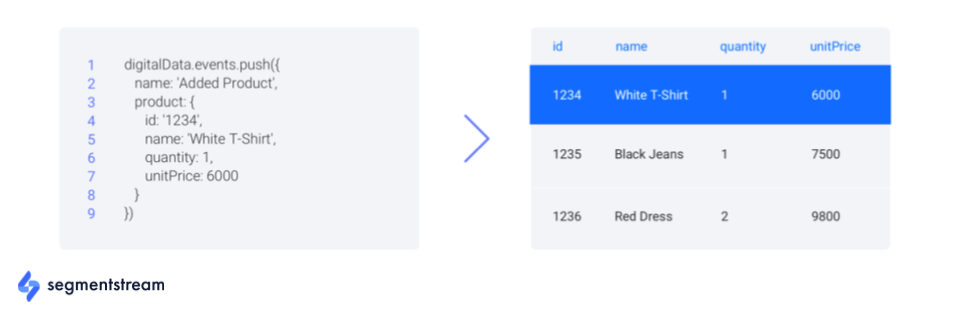
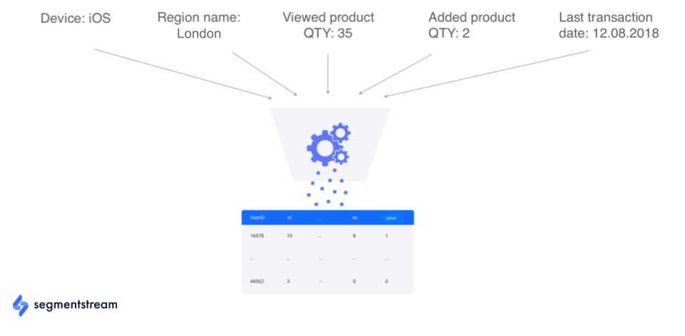
Once raw data is collected, it should be processed into attributes, where every session has a set of features (e.g., device type) and a label (e.g., a purchase in the next 7 days):
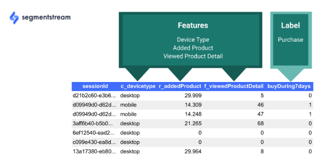
This dataset can now be used to train a model that will predict the probability of making a purchase in the next 7 days.
Step 2: Training a model
In the days before Google BigQuery machine learning, training a model was a complex data engineering task, especially if you wanted to retrain your model on a daily basis.
You had to move data back and forth from the data warehouse to a Tensorflow or Jupyter Notebook, write some Python or R code, then upload your model and predictions back to the database:

With Google BigQuery ML, that’s not the case anymore. Now, you can collect the data, mine features, train models, and make predictions—all inside the Google BigQuery data warehouse. You don’t have to move data anywhere:
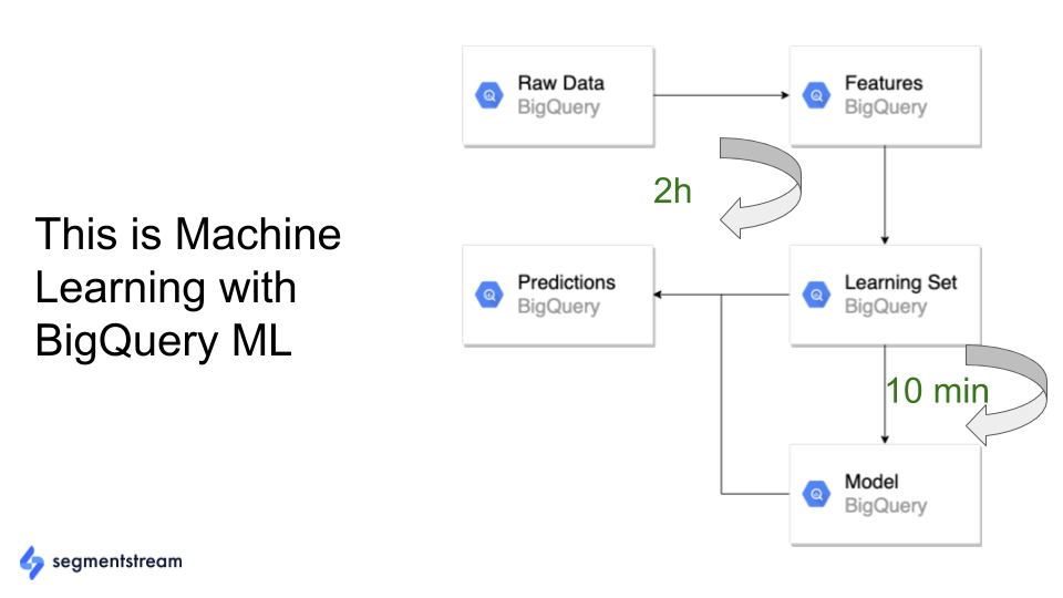
And all of those things can be implemented using some simple SQL code.
For example, to create a model that predicts the probability to buy in the next 7 days based on a set of behavioral features, you just need to run an SQL query like this one*:
CREATE OR REPLACE MODEL`projectId.segmentstream.mlModel`OPTIONS( model_type = 'logistic_reg')AS SELECTfeatures.*labels.buyDuring7Days AS labelFROM`projectId.segmentstream.mlLearningSet`WHERE date BETWEEN 'YYYY-MM-DD' AND 'YYYY-MM-DD'
*Put your own Google Cloud project ID instead of projectId, your own dataset name instead of segmentstream, and your own model name instead of mlModel; mlLearningSet is the name of the table with your features and labels, and labels.buyDuring7Days is just an example.
That’s it! In 30–60 seconds, you have a trained model with all possible non-linear permutations, learning and validation set splits, etc. And the most amazing thing is that this model can be retrained on a daily basis with no effort.
Step 3: Model evaluation
Google BigQuery ML has all the tools built-in for model evaluation. And you can evaluate your model with a simple query (replacing the placeholder values with your own):
   SELECT * FROM
         ML.EVALUATE(MODEL `projectId.segmentstream.mlModel`,
         (
               SELECT
                     features.*,
                     labels.buyDuring7Days as label
               FROM
                     `projectId.segmentstream.mlTrainingSet`
               WHERE
                     date > 'YYYY-MM-DD'
        ),
        STRUCT(0.5 AS threshold)
    )
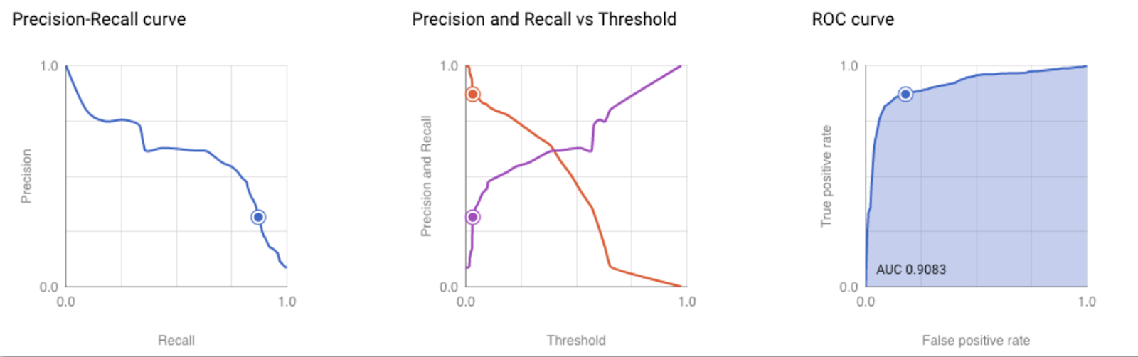
This will visualize all the characteristics of the model:
- Precision-recall curve;
- Precision and recall vs. threshold;
- ROC curve.
Step 4: Building an attribution model
Once you have a model that predicts the probability to buy in the next seven days for each user, how do you apply it to attribution?
A behavior-based attribution model:
- Allocates value to each traffic source;
- Predicts the probability to buy at the beginning and end of the session;
- Calculates the “delta” between the two.
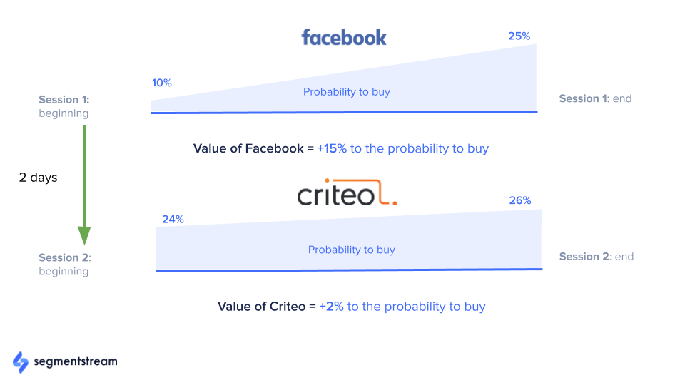
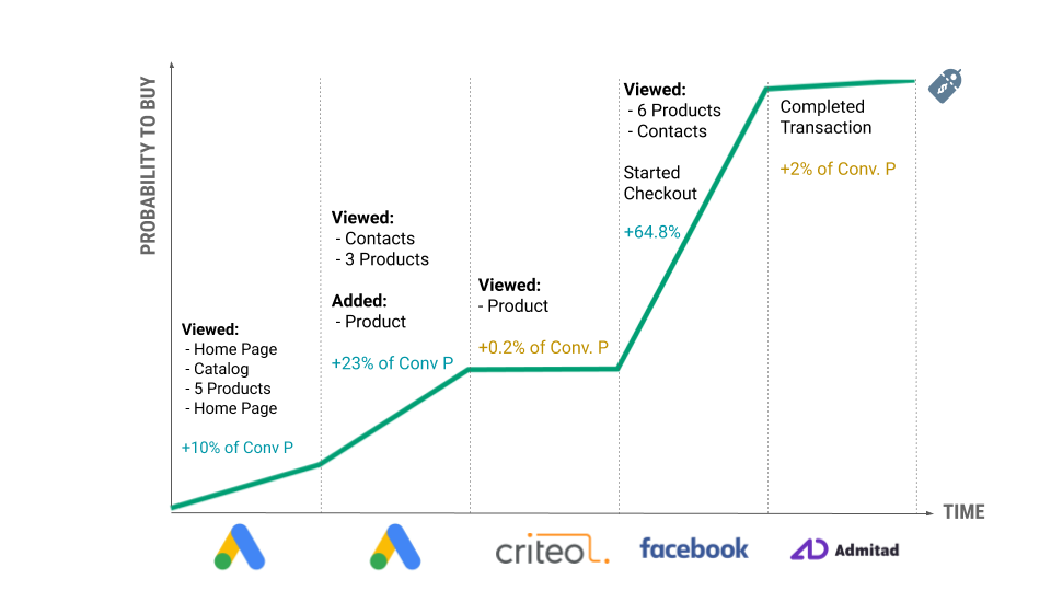
Let’s consider the above example:
- A user came to the website for the first time. The predicted probability of a purchase for this user was 10%. (Why not zero? Because it’s never zero. Even based on contextual features such as region, browser, device, and screen resolution, the user will have some non-zero probability of making a purchase.)
- During the session, the user clicked on products, added some to their cart, viewed the contact page, then left the website without a purchase. The calculated probability of a purchase at the end of the session was 25%.
- This means that the session started by Facebook pushed user probability of making a purchase from 10% to 25%. That is why 15% is allocated to Facebook.
- Then, two days later, the user returned to the site by clicking on a Criteo retargeting ad. During the session, the user’s probability didn’t change much. According to the model, the probability of making a purchase changed only by 2%, so 2% is allocated to Criteo.
- And so on…
In our Google BigQuery database, we have the following table for each user session:
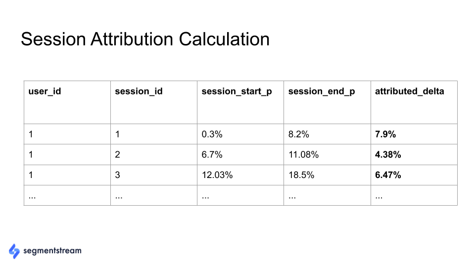
Where:
- session_start_p is the predicted probability to buy in the beginning of the session.
- session_end_p is the predicted probability to buy at the end of the session.
- attributed_delta is the value allocated to the session.
In the end, we have values for all channels/campaigns based on how they impact the users’ probability to buy in the next 7 days during the session:

Tidy as that chart may be, everything comes with pros and cons.
Pros and cons of behavior-based attribution
Pros
- Process hundreds of features as opposed to algorithmic approaches.
- Marketers and analysts have the ability to select domain-specific features.
- Predictions are highly accurate (up to 95% ROC-AUC).
- Models are retrained every day to adapt to seasonality and UX changes.
- Ability to choose any label (predicted LTV, probability to buy in X days, probability to buy in current session).
- No manual settings.
Cons
- Need to set up advanced tracking on the website or mobile app.
- Need 4–8 weeks of historical data.
- Not applicable for projects with fewer than 50,000 users per month.
- Additional costs for model retraining.
- No way to analyze post-view where there is no website visit.
Conclusion
Machine learning still depends on the human brain’s analytical capabilities. Though unmatched in its data processing capabilities, Google BigQuery ML evaluates factors that the user selects—those deemed fundamental for their business based on previous experience.
Algorithms either prove or disprove the hypothesis of the marketer and allow them to adjust the features of the model to nudge predictions in the needed direction. Google BigQuery ML can make that process vastly more efficient.
Related Posts
-

This post is not a dry feature-by-feature comparison, nor does it include a winner-take-all verdict.…
-

When it comes to Google BigQuery, there are plenty of articles and online courses out…
-

After reading some subscriber feedback, we noticed that many CXL readers didn't have a solid…
-

A/B testing tools like Optimizely or VWO make testing easy, and that's about it. They're…

vary good post.