Raise your hand if you’ve ever struggled with a decision between disciplined testing procedures and expedient decision-making.
For example, think of a time when you’ve had to decide between sticking to your A/B test design—namely, the prescribed sample size—and making a decision using what appears to be obvious, or at least very telling, test data. If your arm is waving vigorously in the air right now, this post is for you. Also, put it down and stop being weird.
In my experience, this is a dilemma almost every experimenter faces at one point or another—regardless of company size or traffic count. Time is a cost of running a test, but, in practice, it also represents the cost of continuing a test:
- Forgoing the launch of other experiments;
- Prolonging the exposure of a poor experience;
- Delaying the monetization of a valuable change;
- Sacrificing relationship capital with stakeholders eager to make a decision.
The classic breed of A/B testing methods—known as fixed-horizon tests—assumes that a specific sample size has been committed to in advance; the statistics rely on this assumption for validity.
Many experimenters, however, violate this assumption, peeking at the stats while the test is running and abandoning tests early when results are convincing—introducing unquantified error into their decision-making.
Much has been said on this blog and elsewhere about the evils of peeking. But, by and large, are testers who peek making bad decisions? I wanted to know, so I simulated thousands of tests to find out.
Table of contents
What is textbook peeking, anyway?
I’m not sure we all agree on what peeking looks like. In one article, peeking is defined as calculating p-values after each observation is added to the sample. The article states that under these conditions, 77% of flat, zero-difference tests reached 90% confidence. The author—a smart, experienced guy—was trying to prove a point: you peek, you get more errors.
But what if most peeking doesn’t actually look like this? What if peeking looks more like periodic evaluation every few days while a test is running?
In my simulations, I looked at what would happen if you peeked at every 10% of sample increments. In other words, I designed a test by the book with a fixed sample size, then calculated p-values after simulating the traffic in 10% chunks.
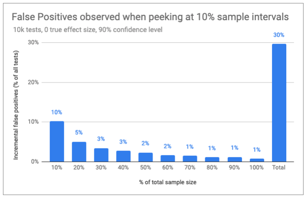
Assuming that you stop the test after observing a significant result, what I found was that 30% of zero-difference (one-tailed) tests reported a false positive using 90% confidence. Obviously, that’s not great. But other lessons were more valuable—and surprising.
Takeaways from 10,000 simulations
1. When you peek makes a difference in error rates.
We know that, in smaller sample sizes, observed effects (the difference between the control and the test) are much more widely distributed. So what if when you peek determines a lot about what you’re likely to see?
You don’t have to be a big football fan to intuit that the team that’s ahead at the end of the first quarter is less likely to win than a team that’s ahead by a wide margin at halftime.
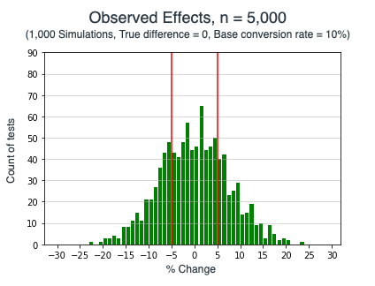
It stands to reason that the same holds true for A/B tests—the more data you collect, the better your predictions become and potentially the more costly it is to continue testing.
So what happens if you don’t peek until after halftime? In simulations that waited until 60% of the sample had been collected for the first peek, and then checking confidence every 10% of sample collected, I saw the rate of false positives under the null fall from 30% to 18%.
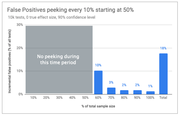
Remember, that’s with 90% confidence, meaning that the expected rate of false positives at the end of the test is 10% when the null hypothesis (difference = 0) is actually true.
But what if the important factor is how many times you peek and not when that peeking occurs? For example, what if instead of peeking four times starting at 60%, we peeked 4 times at the front end of the test, starting at 10%?
It’s hard to see this ever happening in real life, but for the sake of science, let’s have a look.
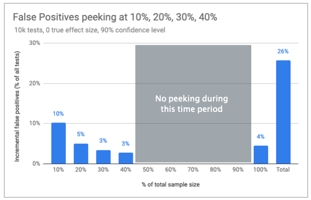
Peeking early, rather than later on, has increased our overall error rate from 18% to 26%. Clearly, timing matters. In fact, the closer your peeking gets to your final analysis, the lower your error inflation becomes.
That said, halftime is a fairly arbitrary place to begin keeping score. The chart below shows how many tests will—at some point—reach confidence, depending on when you begin peeking.
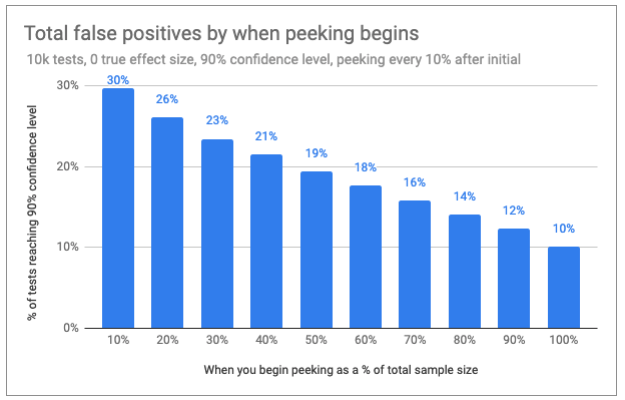
It’s a fairly straight line of decreasing errors start to finish—no magical inflection point at which the impact of peeking clearly diminishes.
The goal here isn’t to find the optimal time to peek but rather to tug on the bedsheet covering the statistical ghost that’s haunted CRO since before Adobe Target was Offermatica.
2. Negative effects are unlikely to produce high confidence after halftime.
As you might imagine, false positives drop further when the truth is a decline in conversion rate. At -2.5% (9.75% against a 10% base conversion rate), only 2.6% of tests produce a false positive result when the first peek occurs at 60% of sample collection.
Here’s the same chart as above repeated for negative effects:
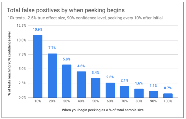
We see that peeking late in the game—even intermittently—may more than triple the number of false positives, but that’s on a very small base. The likelihood of getting a false positive when there’s even a modest drop in conversion rate is not very high in later stages of the test.
That’s good news for any peekers who are willing to risk the occasional flat result or slight decrease to take advantage of shorter run times while avoiding any large declines.
If this thinking revs your engines, you should check out non-inferiority testing for a relatively easy way to model your approach.
3. Positive effects ≥ your MDE rarely reach high confidence if flat at halftime.
The other point of interest to peekers is whether there are strong signals in the early data to suggest that the null hypothesis is true (i.e. that your test variant is very unlikely to be better than the control).
Take a situation where, halfway through a test, we see no difference in performance. How likely is it that we’ve got a sleeping giant versus a dud that makes continuing the test futile?
In my exploration, I simulated tests in which the true effect is a 5% increase in conversion rate (again, on a baseline of 10% with 80% power in the test design). Five percent was also the MDE, so it represents the smallest improvement I sought to detect with high probability.
In this case, I was looking for a reason to give up on the test. If I found confidence to be lower than 55%, I took that as a potential good reason. This would happen only if observed differences were very small or negative.
Below, I’ve charted the results. I’ve broken the data out by tests that exhibit futility early on but then reverse course to display their true colors as a winner by the end of the test.
This group of “recovered tests” represents the true opportunity cost of ending a test for futility at an early stage.
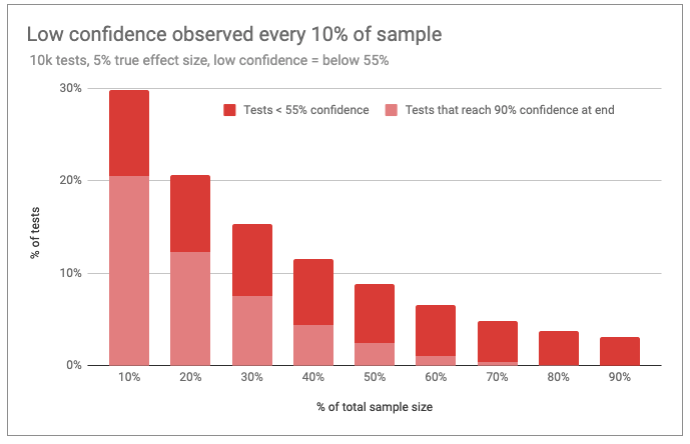
A few things stand out. First, the occurrence of very low confidence levels drops precipitously until about 50% of the sample has been collected. More importantly, however, very few tests exhibiting low confidence from 50% onward ever recover in time to be considered a “win.”
So, what if you delay peeking until the 60% mark, then check every 10% and end the test for futility if confidence drops below 55%? The end result would be abandoning 9% of these true winners before the end, most at the 60% mark.
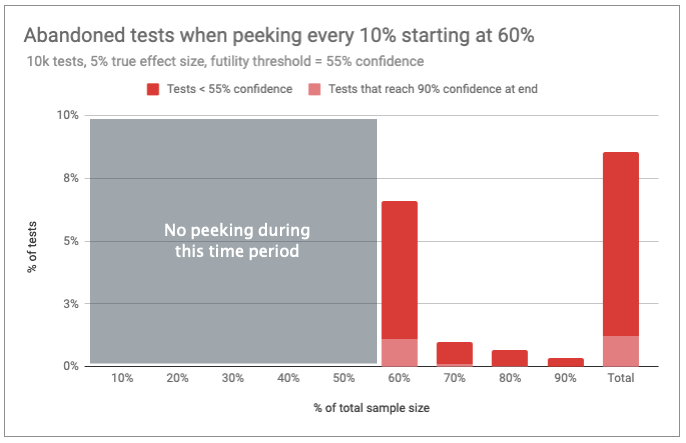
These tests were designed to run with 80% power, meaning that they would fail to detect a 5% increase no more than 20% of the time. Since some of these would have ultimately recovered, you’ll end up reducing your power from 80% to 79%.
Again, this is good news for peekers. Even though 55% confidence is a pretty arbitrary cutoff, giving up on a dud might not be such a bad idea if it means you have more test budget for other ideas.
So it’s okay to peek?
Fixed-horizon testing methods aren’t always efficient. There’s usually very little information to inform what to expect in terms of an effect size, so selecting an MDE can be difficult:
- Select one too low—relative to the actual effect—and your test may be way over-powered, which means collecting a much larger sample than necessary to inform a decision.
- Select one too high, and you won’t stand much of a chance to gather conclusive evidence.
Of course, both scenarios assume that there’s a difference in test groups. Even when there was none in my simulations, it sure seemed like there were reliable signals in the data well ahead of the planned sample sizes.
While our intuitions are not wholly reliable, they’re not always wrong, either. When we’re well into a test and we see extreme results, we’re not wrong to think that a devotion to statistical fidelity might hold us back from an easy decision.
And even if that decision comes back to bite us, that bite doesn’t look too venomous from some of the standpoints we’ve considered here.
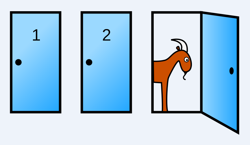
But before you commit to your intuition over the science of statistics, check out the Monty Hall problem for a humbling reminder of our cognitive limitations.
Sequential testing: A better solution
Many online experimentation experts have replaced fixed horizons with sequential and/or Bayesian test methods.
These methods are known as the “right” way to peek under repeated testing conditions. They allow experimenters to make sound decisions in the face of extreme data and, therefore, play the game more efficiently (without violating the assumptions made in their test design).
Experimentation tool providers such as Optimizely, VWO, and Google Optimize—as well as experimentation thought-leaders like Evan Miller, Georgi Georgiev, and Ton Wesseling—are just a few of those who have adopted Bayesian or sequential testing methods.
That’s fine and well for those who have teams equipped to understand and deploy such methods.
While fixed-horizon experimentation concepts are taught in introductory statistics courses, and the availability of online calculators and tutorials is plentiful, the same cannot be said about methods provisioning for intermittent analysis. Most sequential testing concepts are complex, even inaccessible, for the uninitiated.
Not everyone has a data scientist designing and analyzing their experiments. There are many CROs who are a one-stop shop for testing at their organizations and have backgrounds in business or computer science, not math.
If you’re one of these, you may be wondering if the peeking heuristics I’ve shared here are your best alternative. Before you jump to a conclusion, let me suggest a few alternatives.
Sequential testing options for the non-data scientist
Sequential testing refers to a family of methods developed and honed over the past century. Again, the primary purpose of these methods is to control errors in the presence of intermittent analysis and early decisions during data collection.
For a simple sequential option, see Evan Miller’s simple sequential method and accompanying free calculator. You may, like me, find this to impose an odd framing on your analyses.
Another option is to use one of the ready-made test analysis frameworks I offer below. These cover the most common test designs in use today and provide four checkpoints during the test, one after each 25% of your sample has been collected.
You start with a typical 80% power, one-tail test using your choice of 90% or 95% confidence levels and any base conversion rate and MDE. Create your initial test plan, including your sample size (as per normal).
During the test, at each 25% checkpoint, calculate your test statistic (z-score) or p-value as you normally would. Then, compare your value to the decision boundaries in the table below.
If your value stays between the futility (lower) and efficacy (higher) boundaries, continue your test. If your values fall outside these boundaries, end the test—you’re done!
95% Confidence, 80% power, one-tail (with a 9.67% maximum increase in sample size)

90% Confidence, 80% power, one-tail (with a 10.6% maximum increase in sample size)

There is one “gotcha.” To use these designs, you must increase your target sample size by about 10%. To be precise, add 10.6% for 90% confidence and 9.67% for 95% confidence. This is just a total potential or maximum—most tests will never reach the max sample size.
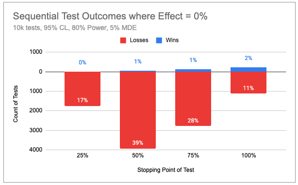
In a simulation of 10,000 flat (no effect) tests that used the 95% confidence model provided, 57% were halted before or at midpoint. Even with the longer maximum duration, sequential tests were 34% shorter than their fixed-horizon equivalents.
As you can see in the chart below, false positives came in very close to our 5% design intention.
In another simulation, in which the effect size was exactly equal to the 5% MDE, 29% of tests ended before or at the midpoint, with an 18% overall savings in sample size. Once again, false negatives were kept in check at 20%, as intended by the design.
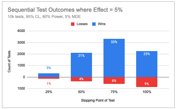
When true effects are between 0 and your MDE, the test is more likely to run to the maximum sample size. But when the effect is less than 0 or greater than the MDE, your average test will be significantly shorter.
That’s exactly what we want: the ability to make early decisions when the impact is more extreme than anticipated.
Tradeoffs in sequential testing
WARNING: If you use this method, you should not attempt to calculate confidence intervals, estimate effect sizes, or report confidence percentage as you normally do. These values must be adjusted to remain accurate given a sequential test design.
Even though you’re using p-values to determine whether the results are statistically significant, those p-values no longer represent true confidence levels.
This highlights the fact that sequential methods are generally much more complex than their run-of-the-mill counterparts. Between this reality—and the fact that the max sample size may actually be longer than for a fixed design—it’s understandable that some experts still shy away from sequential testing.
It’s beyond the scope of this article to detail these alternative procedures and represents a sacrifice you’ll have to make to use this quick-and-dirty method.
Additionally, even though you may be able to identify statistically significant results early on, you must still account for seasonality and business cycles. Most experts recommend running a test for a minimum of 7–14 days to cover a few cycles of day-of-week behavioral differences.
On the bright side, even these simple frameworks empower you to run sequential testing like a pro. Your errors will remain in check, and you can save up to 73% of your required sample size.
Next-level sequential testing
I’ve used the R package gsDesign along with the methods described here to create these test designs. These align closely with the approach employed by Georgi Georgiev’s AGILE test methodology, without a few bells and whistles.
If you’re starting from scratch but are interested in going deeper into the world of sequential test design and analysis, I can tell you that you probably have a lot of work ahead—there are myriad approaches, and some of the computations require software.
The technical process to design and execute a test looks like this:
Pre-test:
- Decide on test parameters (confidence level, power, etc.) and how many times you want to check in on the data.
- Decide which alpha/beta spending functions you want to use. (There are different approaches to modeling the shape of the decision boundaries.)
- Calculate decision boundary values and maximum adjusted sample size.
During test:
- Recalculate decision boundary values throughout the test to correspond with actual checkpoints.
- Calculate z-score and p-values as per normal and compare to decision-boundary values.
- When a boundary is crossed, calculate adjusted p-values and confidence intervals.
Conclusion
As we’ve seen, a more flexible approach to ending tests offers clear efficiencies. That efficiency comes at a cost of added complexity and potentially extending tests longer than a fixed design, but these are worthwhile methods to add to your optimization arsenal.
If these were a challenge to understand, don’t worry. Experimentation isn’t easy, and most of us have to struggle through new methods. Even those who have made a career of understanding p-values have a hard time knowing exactly what they mean.
You can be a brilliant data scientist and not know the first thing about sequential testing. So stick with it. Worth an experiment, anyway, right?
Author’s note: This article benefited from substantial contributions from reviewers, including Georgi Georgiev, Matt Gershoff, Chad Sanderson, and Kelly Wortham. Many thanks to them and to others upon whose work this article builds.




One of the best posts I’ve read lately. Once a person who achieved a lot in life was asked what is the secret of his success. He replied: “I embarked on a small, innocent self-deception. He pretended that the enterprise belonged to me alone, no matter where I worked. I just thought that everything was mine here”. You should never make decisions for which you are not fully responsible. Refusal to make a decision is also a decision. If you have evaluated all the available information and thought overall the likely consequences of your choice, do not stop halfway and make a decision. The only way to avoid mistakes is to do nothing at all. In order to learn how to make decisions wisely, you must be prepared in advance in advance that your reputation may suffer. Thanks and good luck!