Statistical Power: What It Is and How To Calculate It in A/B Testing

Years ago, when I first started split-testing, I thought every test was worth running. It didn’t matter if it was changing a button color or a headline—I wanted to run that test.

My enthusiastic, yet misguided, belief was that I simply needed to find aspects to optimize, set up the tool, and start the test. After that, I thought, it was just a matter of awaiting the infamous 95% statistical significance.

I was wrong.

After implementing “statistically significant” variations, I experienced no lift in sales because there was no true lift—“it was imaginary.” Many of those tests were doomed at inception. I was committing common statistical errors, like not testing for a full business cycle or neglecting to take the effect size into consideration.

I also failed to consider another possibility: That an “underpowered” test could cause me to miss changes that would generate a “true lift.”

Understanding statistical power, or the “sensitivity” of a test, is an essential part of pre-test planning and will help you implement more revenue-generating changes to your site.

What is statistical power?

Statistical power is the probability of observing a statistically significant result at level alpha (α) if a true effect of a certain magnitude is present. It allows you to detect a difference between test variations when a difference actually exists.

Statistical power is the crowning achievement of the hard work you put into conversion research and properly prioritized treatment(s) against a control. This is why power is so important—it increases your ability to find and measure differences when they’re actually there.

Statistical power (1 – β) holds an inverse relationship with Type II errors (β). It’s also how to control for the possibility of false negatives. We want to lower the risk of Type I errors to an acceptable level while retaining sufficient power to detect improvements if test treatments are actually better.

Finding the right balance, as detailed later, is both art and science. If one of your variations is better, a properly powered test makes it likely that the improvement is detected. If your test is underpowered, you have an unacceptably high risk of failing to reject a false null.

Before we go into the components of statistical power, let’s review the errors we’re trying to account for.  

Type I and Type II errors

Type I errors

A Type I error, or false positive, rejects a null hypothesis that is actually true. Your test measures a difference between variations that, in reality, does not exist. The observed difference—that the test treatment outperformed the control—is illusory and due to chance or error.

The probability of a Type I error, denoted by the Greek alpha (α), is the level of significance for your A/B test. If you test with a 95% confidence level, it means you have a 5% probability of a Type I error (1.0 – 0.95 = 0.05).

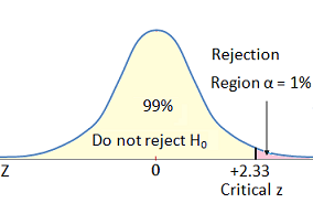
If 5% is too high, you can lower your probability of a false positive by increasing your confidence level from 95% to 99%—or even higher. This, in turn, would drop your alpha from 5% to 1%. But that reduction in the probability of a false positive comes at a cost.

By increasing your confidence level, the risk of a false negative (Type II error) increases. This is due to the inverse relationship between alpha and beta—lowering one increases the other.

Lowering your alpha (e.g. from 5% to 1%) reduces the statistical power of your test. As you lower your alpha, the critical region becomes smaller, and a smaller critical region means a lower probability of rejecting the null—hence a lower power level. Conversely, if you need more power, one option is to increase your alpha (e.g. from 5% to 10%).

Type II errors

A Type II error, or false negative, is a failure to reject a null hypothesis that is actually false. A Type II error occurs when your test does not find a significant improvement in your variation that does, in fact, exist.

Beta (β) is the probability of making a Type II error and has an inverse relationship with statistical power (1 – β). If 20% is the risk of committing a Type II error (β), then your power level is 80% (1.0 – 0.2 = 0.8). You can lower your risk of a false negative to 10% or 5%—for power levels of 90% or 95%, respectively.

Type II errors are controlled by your chosen power level: the higher the power level, the lower the probability of a Type II error. Because alpha and beta have an inverse relationship, running extremely low alphas (e.g. 0.001%) will, if all else is equal, vastly increase the risk of a Type II error.

Statistical power is a balancing act with trade-offs for each test. As Paul D. Ellis says, “A well thought out research design is one that assesses the relative risk of making each type of error, then strikes an appropriate balance between them.”

When it comes to statistical power, which variables affect that balance? Let’s take a look.

The variables that affect statistical power

When considering each variable that affects statistical power, remember: The primary goal is to control error rates. There are four levers you can pull:

1. Sample size
2. Minimum Effect of Interest (MEI, or Minimum Detectable Effect)
3. Significance level (α)
4. Desired power level (implied Type II error rate)

1. Sample Size

The 800-pound gorilla of statistical power is sample size. You can get a lot of things right by having a large enough sample size. The trick is to calculate a sample size that can adequately power your test, but not so large as to make the test run longer than necessary. (A longer test costs more and slows the rate of testing.)

You need enough visitors to each variation as well as to each segment you want to analyze.  Pre-test planning for sample size helps avoid underpowered tests; otherwise, you may not realize that you’re running too many variants or segments until it’s too late, leaving you with post-test groups that have low visitor counts.

Expect a statistically significant result within a reasonable amount of time—usually at least one full week or business cycle. A general guideline is to run tests for a minimum of two weeks but no more than four to avoid problems due to sample pollution and cookie deletion.

Establishing a minimum sample size and a pre-set time horizon avoids the common error of simply running a test until it generates a statistically significant difference, then stopping it (peeking).

2. Minimum Effect of Interest (MEI)

The Minimum Effect of Interest (MEI) is the magnitude (or size) of the difference in results you want to detect.

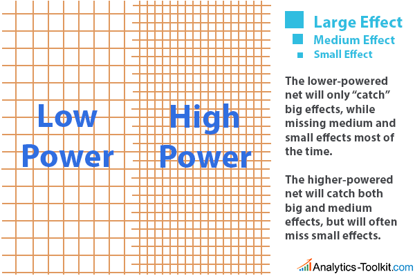
Smaller differences are more difficult to detect and require a larger sample size to retain the same power; effects of greater magnitude can be detected reliably with smaller sample sizes. Still, as Georgi Georgiev notes, those big “improvements” from small sample sizes may be unreliable:

The issue is that, usually, there was no proper stopping rule nor fixed sample size, thus the nominal p-values and confidence interval (CI) reported are meaningless. One can say the results were “cherry-picked” in some sense.

If there was a proper stopping rule or fixed sample size, then a 500% observed improvement from a very small sample size is likely to come with a 95% CI of say +5% to +995%: not greatly informative.

A great way to visualize the relationship between power and effect size is this illustration by Georgiev, where he likens power to a fishing net:

3. Statistical Significance

As Georgiev explained:

An observed test result is said to be statistically significant if it is very unlikely that we would observe such a result assuming the null hypothesis is true.

This then allows us to reason the other way and say that we have evidence against the null hypothesis to the extent to which such an extreme result or a more extreme one would not be observed, were the null true (the p-value).

That definition is often reduced to a simpler interpretation: If your split-test for two landing pages has a 95% confidence in favor of the variation, there’s only a 5% chance that the observed improvement resulted by chance—or a 95% likelihood that the difference is not due to random chance.

“Many, taking the strict meaning of ‘the observed improvement resulted by random chance,’ would scorn such a statement,” contended Georgiev. “We need to remember that what allows us to estimate these probabilities is the assumption the null is true.”

Five percent is a common starting level of significance in online testing and, as mentioned previously, is the probability of making a Type I error. Using a 5% alpha for your test means that you’re willing to accept a 5% probability that you have incorrectly rejected the null hypothesis.

If you lower your alpha from 5% to 1%, you are simultaneously increasing the probability of making a Type II error, assuming all else is equal. Increasing the probability of a Type II error reduces the power of your test.

4. Desired Power Level

With 80% power, you have a 20% probability of not being able to detect an actual difference for a given magnitude of interest. If 20% is too risky, you can lower this probability to 10%, 5%, or even 1%, which would increase your statistical power to 90%, 95%, or 99%, respectively.

Before thinking that you’ll solve all of your problems by running tests at 95% or 99% power, understand that each increase in power requires a corresponding increase in the sample size and the amount of time the test needs to run (time you could waste running a losing test—and losing sales—solely for an extra percentage point or two of statistical probability).

So how much power do you really need? A common starting point for the acceptable risk of false negatives in conversion optimization is 20%, which returns a power level of 80%.

There’s nothing definitive about an 80% power level, but the statistician Jacob Cohen suggests that 80% represents a reasonable balance between alpha and beta risk. To put it another way, according to Ellis, “studies should have no more than a 20% probability of making a Type II error.”

Ultimately, it’s a matter of:

• How much risk you’re willing to take when it comes to missing a real improvement;
• The minimum sample size necessary for each variation to achieve your desired power.

How to calculate statistical power for your test

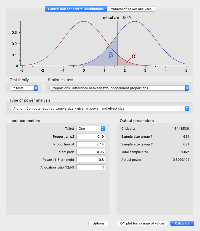
Using a sample size calculator or G*power, you can plug in your values to find out what’s required to run an adequately powered test. If you know three of the inputs, you can calculate the fourth.

In this case, using G*Power, we’ve concluded that we need a sample size of 681 visitors to each variation. This was calculated using our inputs of 80% power and a 5% alpha (95% significance). We knew our control had a 14% conversion rate and expected our variant to perform at 19%:

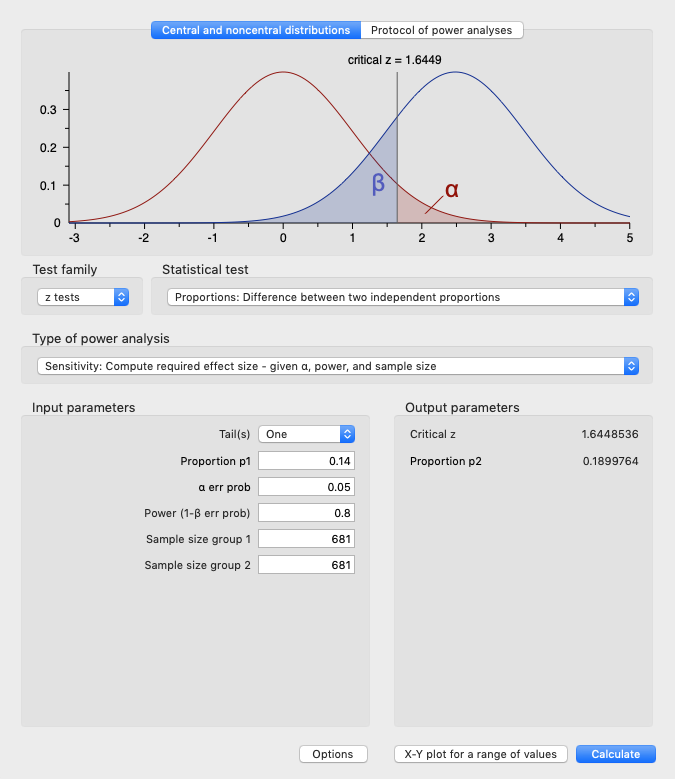
In the same manner, if we knew the sample size for each variation, the alpha, and the desired power level (say, 80%), we could find the MEI necessary to achieve that power—in this case, 19%:

What if you can’t increase your sample size?

There will come a day when you need more power but increasing the sample size isn’t an option.  This might be due to a small segment within a test you’re currently running or low traffic to a page.

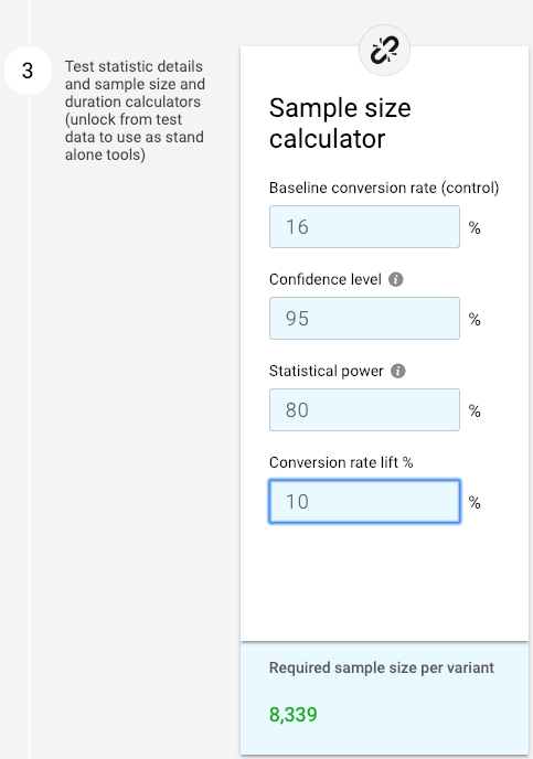
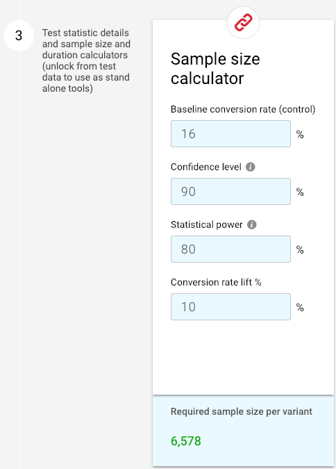
Say you plug your parameters into an A/B test calculator, and it requires a sample size of more than 8,000:

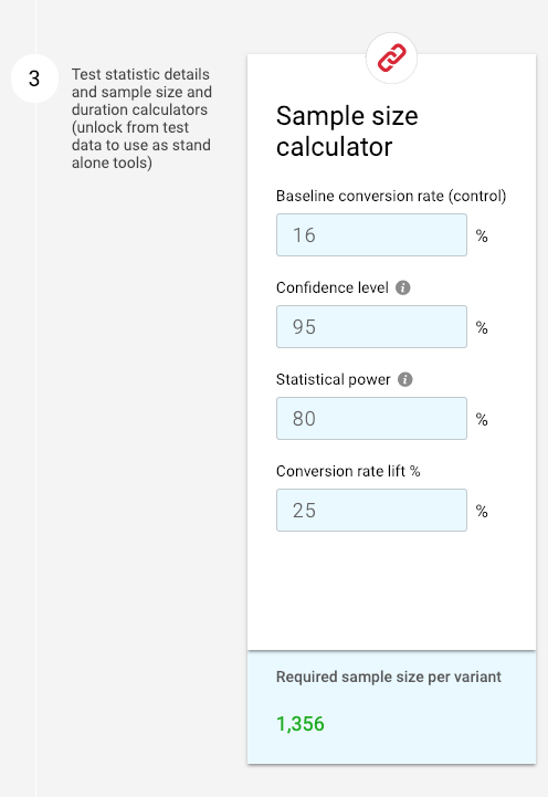
If you can’t reach that minimum—or it would take months to do so—one option is to increase the MEI. In this example, increasing the MEI from 10% to 25% reduces the sample size to 1,356 per variant:

But how often will you be able to hit a 25% MEI? And how much value will you miss looking only for a massive impact? A better option is usually to lower the confidence level to 90%—as long as you’re comfortable with a 10% chance of a Type I error:

So where do you start? Georgiev conceded that, too often, CRO analysts “start with the sample size (test needs to be done by <semi-arbitrary number> of weeks) and then nudge the levers randomly until the output fits.”

Striking the right balance:

• Requires a thoughtful process as to which levers to adjust;
• Benefits from measuring the potential change in ROI for any change to test variables.

Conclusion

Statistical power helps you control errors, gives you greater confidence in your test results, and greatly improves your chance of detecting practically significant effects.

Take advantage of statistical power by following these suggestions:

1. Run your tests for two to four weeks.
2. Use a testing calculator (or G*Power) to ensure properly powered tests.
3. Meet minimum sample size requirements.
4. If necessary, test for bigger changes in effect.
5. Use statistical significance only after meeting minimum sample size requirements.
6. Plan adequate power for all variations and post-test segments.

Working on something related to this? Post a comment in the CXL community!